Waiting on Tests
Disclaimer: views expressed are my own and are not endorsed by my employer.
In 2019 we had roughly zero automated tests at StrongDM. We did manual quality assurance testing on every release. Today we have 56,343 tests.
Anecdotally, the rate of bugs and failures has not decreased by a commensurate amount. Instead I think it correlates with focused efforts we’ve made at various times to either ship big new features (resulting in many unforeseen bugs), or stabilize existing features (resulting in fewer bugs).
When trying to determine whether a new feature is working, I think automated tests are only marginally more effective than manual QA testing. But once that feature is done, we want to make sure it keeps working, and that’s where automated tests save a lot of time.
So in my opinion, the primary purpose of automated tests is not to avoid failures, but to speed up development. Which means a slow test suite defeats its own purpose. So I try to optimize our tests whenever I get the chance. Here’s some recent work I did in that vein.
The starting line
On a good day in September 2023, a test run might look like this if you’re lucky:
Initialization     Waited 8s     Ran in 51s

(In parallel:)

job1               Waited 10s    Ran in 6m42s
job2               Waited 3s     Ran in 4m13s
job3               Waited 5s     Ran in 4m4s
job4               Waited 2s     Ran in 4m31s
job5               Waited 5s     Ran in 8m54s
job6               Waited 43s    Ran in 6m4s
job7               Waited 44s    Ran in 5m14s
job8               Waited 46s    Ran in 2m43s
job9               Waited 47s    Ran in 4m28s
job10              Waited 48s    Ran in 1m57s
job11              Waited 59s    Ran in 54s

Passed in 9m50s
After the initialization step, the CI pipeline kicks off 11 parallel jobs, each on a separate machine. Very frequently, these jobs stretch out to 12-15 minutes.
In October, I did a lot of optimizations and improvements that I won’t cover here. They should have sped things up a lot, but the needle just wasn’t moving. I hit a wall.
Fingering the culprit
If you look again at the test run above, you’ll notice that some of the jobs say something like “Waited 5s”, while others are more like “Waited 45s”. The former run instantly because there’s already a build server available; the latter have to wait on our Auto-Scaling Group (ASG) to spin up a new build server.
If you zoomed in on one of these jobs on a brand new build server, you would notice another delay caused by cloning the Git repo from scratch, and another delay from downloading Docker images. It all adds up to over three minutes before a single test can run. And after all that, the tests themselves are slower on these fresh instances since the Go build cache is empty.
So the culprit is, freshly launched build servers take longer to run tests.
Our ASG was configured to keep a minimum of four c5d.4xlarge instances hot and ready during working hours, with the ability to add more as needed. Extra instances above the minimum would wait for jobs for ten minutes and then timeout and shutdown. On nights and weekends it all scaled to zero.
The critical realization is that it doesn’t matter if four of the eleven jobs finish super fast; we still have to wait on the slowest job. So there’s no point keeping those four instances running. We might as well scale down to zero between test runs. Maybe we should do that and increase the shutdown timeout to twenty minutes.
The knobs
The ASG has two knobs we can adjust:
- The minimum instance count (currently four)
- The timeout - how long each instance waits for work before shutting down (currently ten minutes)
I wanted to minimize the number of “cold starts”, where a cold start is any time a developer kicks off a test and has to wait for at least one new build server to boot up.
I also wanted to minimize cost, where cost is, well, money.
So what are the optimal values for these two knobs?
Collecting data
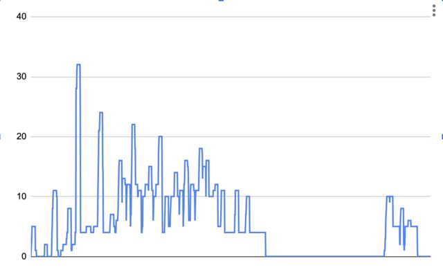
First I needed to understand the status quo. I found a “Desired instance count” metric in Cloudwatch that tracks how many instances our ASG is supposed to be running for every minute of the day. It looked like this on a typical day:
You can easily see the four instance shelf during working hours.
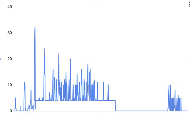
Note that this is the desired instance count. The actual instance count looked more like this:
Each peak gets stretched out at least ten minutes, because the instances wait around that long to see if there’s more work before shutting off.
Trying science
I’ve never used a Jupyter notebook before, but I thought it would be the perfect tool to solve this problem. Turns out, you can use Jupyter right in your browser. I loaded the graph in JSON and tried to calculate how much we were currently spending.
Basically I needed to calculate the area under the above graph. This turned out to be easy because the dataset had exactly one entry per minute, so I just summed up the entries:
import json

f = open('asg_stats.json')

time_series = json.load(f)

# c5d.4xlarge on demand in us-west-2 = $0.768 hourly
on_demand_cost_per_minute = 0.768 / 60.0
work_days_per_month = 22.0

monthly_cost = sum(x for x in time_series) * on_demand_cost_per_minute * work_days_per_month
It’s even easier to calculate the number of cold starts. Any time the instance count increases, that’s a cold start:
cold_starts = sum(1 if time_series[x] < time_series[x+1] else 0 for x in range(len(time_series)-1)) * work_days_per_month
I got $2,220.98 and 2,486 cold starts per month.
Building the simulation
To see what would happen if I increase the minimum instance count to N, I can make sure every entry within working hours is at least N, and then re-run my calculation.
Rather than figuring out dates and times, I checked if each entry was four or more (the current minimum), and if so, bumped it up to at least N.
def min_asg_size(time_series, floor):
    result = [x for x in time_series]
    for i in range(len(result)):
        if result[i] >= 4:
            result[i] = max(result[i], floor)
    return result
Trying out a timeout value of N minutes is made easy again by our dataset having one entry per minute. I just set the current entry to the maximum value of the last N entries.
def shutdown_timeout(time_series, shutdown_timeout_minutes):
    result = [x for x in time_series]
    for i in range(len(result)):
        for j in range(i, min(i+shutdown_timeout_minutes, len(result))):
            result[j] = max(result[j], time_series[i])
    return result
Using Jupyter
I am not a data scientist. If you are one, I apologize for this next part.
I formulated the problem in terms of a single “efficiency” function, which I could then analyze to find the maximum value. I decided to add together the cold start count and the monthly cost, compare that to the status quo, and negate it so that lower costs and cold starts results in higher efficiency. This definition of efficiency assumes that it’s worth it to spend one extra dollar per month if it prevents one cold start per month.
Then I defined a reasonable domain of possible values for my two variables:
array = [
	[timeout for timeout in range(0, 30)]
	for min_instances in range(0, 25)
]
For each one of these configurations, I ran the dataset through my simulation and calculated the efficiency for that entry.
Then I tried to make a graph of this.
The code for this was a bit cryptic, something about ax.imshow() and plt.subplot().
The internet offered millions of conflicting tutorials.
But with trial and error I eventually got something.
At the top I made it spit out the status quo configuration, the best possible configuration, and a hand-picked “Plan B” which was a bit cheaper if needed.
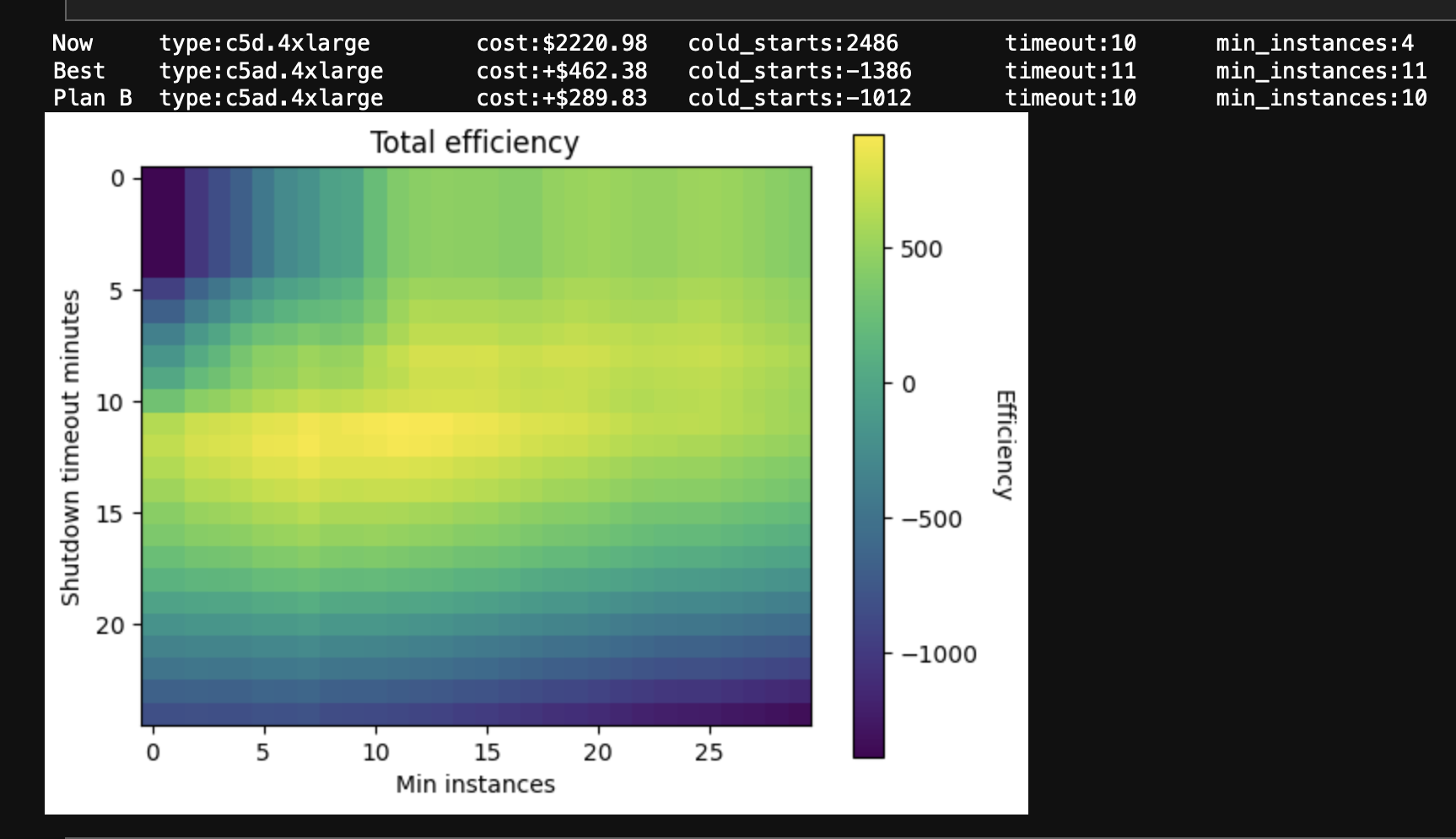
The shutdown timeout was already roughly optimal at ten minutes, but the optimal minimum instance count was eleven. I found this suspiciously close to the numbers required to run the most common test suite: eleven machines for ten minutes. (I would like to re-run this analysis now that the test suite is faster, to see if the optimal timeout stays at ten minutes, or if it scales with the length of the test suite.)
I was surprised that it cost practically the same to more than double the minimum instance count, and that it performed much better than scaling to zero and increasing the timeout.
(It helped that during my research I discovered the c5ad.4xlarge instance type, which gave similar performance at a cheaper price due to the use of AMD processors instead of Intel.)
After all that, the answer ended up being, “have enough build servers on hand to execute the most common set of tests”. It seems so simple in hindsight.
Denouement
So we cut the number of cold starts nearly in half for about the same price.
The nicest part about the Jupyter notebook was sharing it. I pasted it into a secret Github Gist and got a shareable URL with the source code, data, and pretty pictures all in one.
I ended up doing a number of other optimizations:
- Cached
node_modulesin S3. - Tried to cache
GOCACHEin S3 and found it only made things worse. - Cut the most common test run from eleven jobs down to eight.
- Split the longest test jobs into multiple parallel jobs using Buildkite parallelism.
- Optimized and consolidated our Docker images.
- Replaced the expensive and useless Buildkite Test Analytics with a home-grown solution that quickly exposed some unnecessarily slow tests.
- Realized that, despite paying extra for EC2 instances with physical attached SSDs, I was still using a networked EBS volume. 🤦 The physical drives were not mounted automatically like I assumed. (Anecdotally, the SSDs do seem to make a difference.)
A future post might dive into more of that, but for now, tests these days commonly run in under five minutes. 🙌